Contents
Index
Associativity - Building a Transformation Grid
GIS - Solving the Problem of “Associativity”
M.H.Elfick. Research Associate
Dept Civil, Surveying & Environmental Engineering
University of Newcastle Australia
cemhe@cc.newcastle.edu.au
The problem of "associativity" has been the subject of endless papers in GIS/LIS journals – it has been defined by Prof Ian Williamson
as “the association between features in different layers in a layer based GIS/LIS”.
Many GIS packages provide ways to create points and lines in relative position to other features.
However, in most cases, the relativity data is discarded and only the absolute coordinates of the points are stored.
If the base layer is changed at a later date, then the associated points on other layers are no longer
in their correct relative position to the base layer.
For example, telegraph poles may be located by their offset from street boundaries, and at a later date the street
boundaries are changed because a better value for their geographic position is available.
If corrections are not applied to the telegraph pole layer, they will appear to be incorrectly
located with respect to the street boundaries.
As there may be many layers dependent on the base cadastral layer, any changes to that layer have to be allowed for
in all the associated layers.
The main opposition to moving to the NCDB will come from users who have invested considerable resources on
building associated layers based on the DCDB and are worried about the transition process.
If we are building the NCDB, we should also address this problem. One method of solving this problem is by
use of a correction mesh.
Imagine a square mesh overlaying the whole of the area of interest with each node having a correction value
for X and a correction value for Y indicating the relative shift in coordinates between the old and new cadastral
boundaries at that point.
Such a mesh can be generated using similar techniques to those used for forming a grid based digital terrain
model from a table of spot heights only in this case there are two values, one for X corrections and one for Y corrections.
The values needed to build the mesh can be determined by matching the positions of points in the old cadastre with their
corresponding point in the later system.
To update the associated layers, it is only necessary to read each point, look up the corrections in the mesh,
apply the correction and write the point back.
To facilitate the use of GPS, many countries including Australia are revising their geodetic referencing
systems and adopting a world based standard reference ellipsoid for their coordinate systems.
Because of local irregularities in many of the old geodetic survey networks, a direct mathematical transformation
between the old and the new system will not provide results to the required accuracy.
The solution has been to take accurate GPS observations at the major trig points and use these to determine a
correction grid for the local irregularities. The format for this grid and the method of applying it has virtually
become a default standard and there are a variety of public domain packages available to handle many file formats.
So the techniques and the software to solve the problem exists and is being used in Australia and America to
convert coordinates to the new world based systems We can use the same procesures to overcome the “associativity problem”
Because many of the organisations who use the DCDB also have carried out their own updates and upgrades,
there will be many and varied versions of the DCDB. The only reliable method for building a correction grid is to
use data from each organisation to build a grid tailored for their use.
To update associated layers from a DCDB system to a NCDB system I suggest the following:
Export from the DCDB system a table of lines covering the area of interest.
Geodata would have a special utility to read this data, match the lines with their counterparts in the NCDB and
build a correction grid.
This grid would be then be supplied with the NCDB for the client to use to update the associated layers.
The tricky part is the second which will have to be largely automatic because of the size of the data sets.
To demonstrate the practicality of this solution, we have added a module to the program to perform this operation.
It was chosen because it has the capacity to read and write data to most GIS and COGO systems as well as a good
variety of graphics routines.
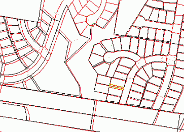
The picture below shows part of a cadastral data set has been read into the program, the red lines are from the
NSW DCDB and the black lines are from a Geodata NCDB. The differences between common lines in the two data sets
range from 0 to 7 metres.
The DCDB data was read in as a series lines and text strings in DXF format. Each text string was the code/lot/plan
identifier used by the LIC and most of these were near to the lot centroid.
The program will automatically built a parcel network out of the lines by creating polygons around each centroid
and named each polygon by the code/lot /plan identifier. This allows the initial matching to take place at the lot
level by matching the identifiers.
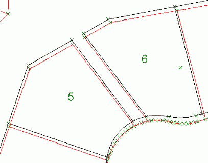
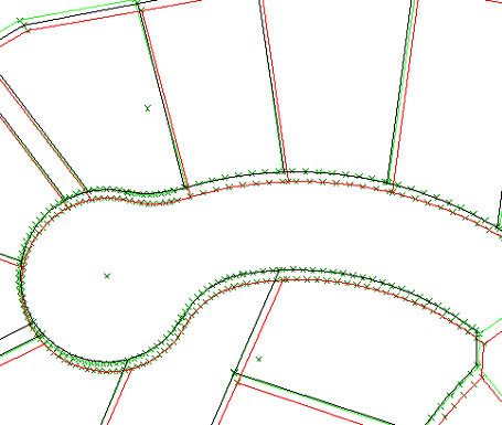
The second picture shows a close up of a section of the job to illustrate the problem of point matching where there
are circular curves. The DCDB represents a curve by a number of short chords and therefore it is difficult to directly
locate the correct matching points.
The solution adopted uses a progressive approach. Points away from the curve are first matched and bad matches
eliminated by "robust estimator" techniques. Then parameters are calculated to transform the DCDB parcel to the NCDB
system and these are used to select the correctly matching points on the curved frontages.
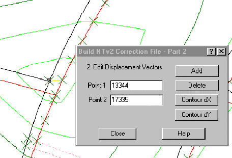
A drop down box allows the user to select the layers to be matched . The difference vectors are calculated and a
contour map drawn showing differences in the X direction. The minor contours are at 200mm intervals and the major
ones are at one metre intervals.
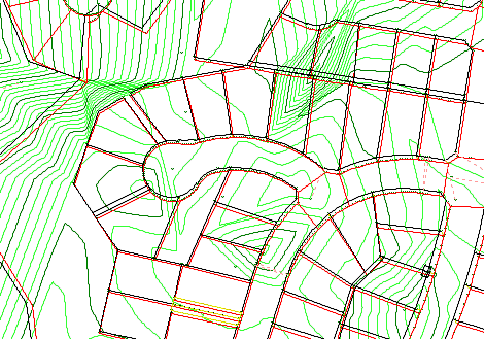
The contours provide a convenient means of assessing the process. Any miss-matches or discontinuities in the cadastral
fabric will show up as "whirlpools" or areas of close contour interval. An edit facility is provided to delete and add
error vectors as needed and to display either dX contours or dY contours.
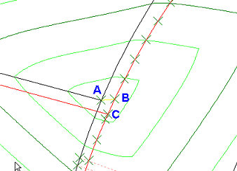
The picture above shows a typical problem. Point A on the NCDB has been connected to point B on the DCDB instead of
being connected to point C. The connecting vector is shown in yellow and there is a "whirlpool around point A.
A "drop down" edit box allows the operator to carry out the changes. Points can be selected by mouse and the screen
can be panned and zoomed to look at any problem in detail.
After the changes have been made, the contours are displayed again to verify that the two layers have been correctly matched.
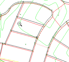
A view of a larger area shows the typical trends in variability of position for parcels in the DCDB and explains
why traditional techniques such as "rubber sheeting" or mathematical operations using polynomial transformations are not appropriate.
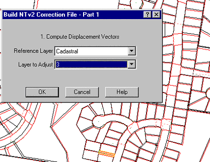
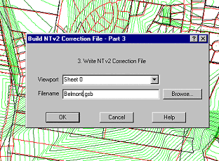
When the area of interest has been matched correctly, a "drop down" box can be displayed to select the file for the correction data
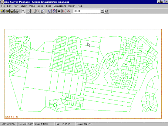
To check the correction grid, a new job can be opened and the DCDB lines read in.
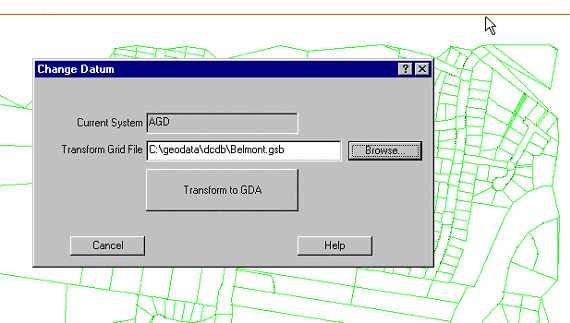
The correction grid can then be applied to the data in the job
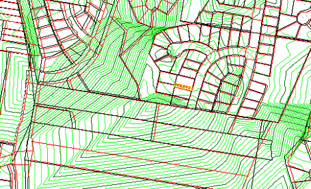
The process can be checked by reading in the old job on top of the transformed DCDB.
Note how the green lines are now superimposed on the black lines (the NCDB) ,. their original position was over
the red lines (the DCDB)
This short example illustrates the principles involved in the process.
Correction files in the NTv2 format can be made up of any number of sub-grids and each sub-grid can be at a
different grid spacing depending on the variability of the data to be transformed. This allows a correction grid
to be assembled by working with the cadastre in manageable "chunks" rather than having to try and work with a large area.
For the above exercise a grid mesh of two seconds of arc on the surface of the earth was used.
This corresponds to about 60 metres in distance. In rural areas the mesh size could probably be relaxed and there may be
urban areas where it may be necessary to reduce it.